A CHEAP AND ACCURATE
FM DEVIATION METER

Written by: Charles A. Bliley, Rochester, New York, 2/4/83

BACKGROUND

This article was written as the result of a complaint. I was working in a radio-electronic company and was an active ham radio operator at the time operating on the two-meter (146 MHz) FM band. The equipment was relative simple and most transceivers had internal transmit deviation adjustment. That was great, but to measure the deviation level was the domain of professionals who owned very expensive deviation meters costing thousands of dollars. The measurement of your transmitter's deviation was impractical for most of us.

One day, I complained to a fellow radio/electronics instructor about my need to measure narrow-band FM deviation. That man was Tom Wise, an electronics engineer turned technical trainer. With abundant help from Tom, we came up with a scheme that would allow an accurate measurement with minimal equipment. Tom explained the principal, I supplied the equipment and off we went on a journey to test the theoretical and make it practical. Below is the article I wrote in 1983 to pass out to a few friends. I sat in my files until March of 2011 when I decided it merited wider circulation via the Internet.

Thank you Tom for your joyful assistance in solving my problem and expanding my knowledge of radio-electronics.

I hope you find it interesting and useful.

Chuck Bliley
Rochester, New York

INTRODUCTION

The two biggest problems with FM and repeater operation are: 1. staying, or getting on, frequency, and 2. too little or too much deviation. With the development of inexpensive frequency counters with fairly good accuracy, only the second problem is left to be tackled.

Because most amateurs can get away without a FM deviation meter, few ever spend the $150 or more to buy one. Nevertheless, safely modulating your FM transmitter to its fullest can give you a bit of a boost when the going gets tough, and signals are weak.

Knowing most amateurs are interested in bargains and care little for high powered mathematics, I will attempt to explain how you can build a setup to accurately measure transmitter deviation with less than a 5% error and spend under $7.00 for the critical parts. In this case, the only critical part is a crystal whose frequency matches your receiver's second IF center frequency. First the boring mathematical part. There exist some mathematical formulas called Bessel Functions " which confuse and frustrate most people, but what they do is show a predictable relationship between the FM signal's modulating frequency and the amount of change in carrier frequency (deviation). These formulas predict for example, with a 1 KHz modulating frequency, at precisely +2.404 KHz deviation, the carrier frequency signal will disappear and only the upper and lower sideband signals will remain.

Now if we can come up with a scheme to find out and measure when the carrier disappears, we can create a deviation meter.

What follows is an inexpensive and fairly easy way to come up with an accurate deviation meter. Be prepared to take on the added responsibility that will come along with being the keeper of the measurement keys. You will soon be tempted to tell others they are under or over deviating with certainty. The power is awesome! Treat it with respect. .

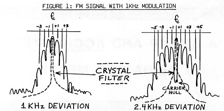
Figure 1: FM Signal with 1kHz Modulation

Figure 1 shows a typical FM signal as observed on a spectrum analyzer test set. Of course an unmodulated carrier would appear only as a single pulse on the screen of the spectrum analyzer's oscilloscope. As we increase the deviation of our 1 KHz modulating tone, sidebands will be created with some carrier level present most of the time. At certain combinations of the modulating frequency and deviation, the carrier will disappear completely from view as shown on the right. With 1 KHz modulation this occurs at 2.404 KHz, 5.520 KHz and at an "infinite" number of other points until the deviation swing equals the carrier frequency.

Table 1: Deviation for FM Carrier Null

One of the problems amateurs have is finding a nice pure 1 KHz modulation source. One kilohertz is a two-way radio standard but, really any frequency in the audio range of a voice will do nicely. Touch Tone encoders are very common with many capable of generating a single pure tone by merely depressing two keys in a row, vertically or horizontally. Table 1 includes seven of the Touch Tone frequencies, plus 1KHz, along with their respective deviation null points. This solves the problem of finding a suitable single tone source, now let's look at how to make the measurements.

FM DEVIATION MEASUREMENT WITH A CRYSTAL FILTER

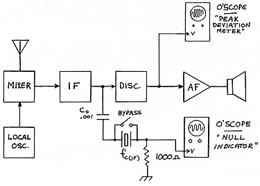
Figure 2. System Set-Up (One oscilloscope will serve double-duty.)

What we want to do is come up with a method of monitoring what is happening on the carrier's frequency of an FM signal and reject all other frequencies. By tapping off the IF signal before the limiter, we can catch the FM signal in its purest form and with a good working level. Next, we attempt to pass the signal through a crystal cut to the center of the receivers IF frequency. The crystal is very selective (typically 20 to 40 HZ at 455 KHz) and will allow only signals falling within its narrow bandpass to pass on to our oscilloscope. The oscilloscope will be used to indicate the level of these signals and as a null indicator during our deviation measurements. Since the crystal is very selective and not tunable, we must first align the source signal's (transmitter's) frequency, or the receiver's first local oscillator, to create a carrier frequency in the receiver's IF precisely equal to the crystal's resonance. By carefully adjusting one oscillator (TX or RX) you can find a point where the unmodulated carrier will peak up nicely on the oscilloscope. Now as the modulation level (deviation) is increased, the null points for the carrier can be measured as indicated by a minimum signal on the oscilloscope. Select a fairly fast sweep which will show less than ten cycles of the carrier signal.

Once you have found the first null point, quickly transfer the oscilloscope to the discriminator output and measure the peak voltage on the scope. You will now be able to relate this peak level on your scope to a deviation level on any incoming signal regardless of modulation frequency or type. Repeat this process with as many modulating frequencies and deviations as necessary to get a sufficient number of calibration points on your screen.

I have selected the discriminator output point for two reasons. First there is no interaction with the volume control, and secondly we want to bypass the effect of the de-emphasis circuit in order to have a flat response for our measurements.

Some people may be interested in measuring deviation at higher frequencies such as 10.7 MHz. I have tried using a 10.7 MHz crystal in this set-up as shown in the block diagram unsuccessfully. Probably this can be attributed to greater path leakage around the crystal and a wider bandwidth for a comparable quality crystal in this higher frequency range

One spin off from the purchase of the 455 KHz crystal could be the building of a test and alignment oscillator as described in the February 1982 issue of QST magazine. By purchasing an additional crystal at 10.7MHz, you could build some inexpensive and practical test equipment for the alignment of your receiver's IFs.

FM DEVIATION MEASUREMENT PROCEEDURE

1. Feed unmodulated signal to be measured into receiver.
2. Set filter switch to bypass.
3. Using an AC coupled oscilloscope, adjust for full scale indication of CW IF signal. Set sweep to show 5 or 10 cycles of IF signal. (The oscilloscope should have reasonable sensitivity at the IF frequency).
4. Open bypass switch.
5. Adjust signal source or receiver LO until receiver IF signal frequency equals the crystal resonance and a peak indication is viewed on the oscilloscope
6. Increase oscilloscope vertical gain until full scale indication is seen. (The filter may create a 3 db loss).
7. Slowly increase modulation of the signal being measured until first and second nulls are measured. Remember - use only a single frequency modulation tone for the calibration process.
   
8. After you have found each null point, move the oscilloscope to the discriminator output and before any deeps circuits. Note the peak output voltage at each null point you want to use for the calibration process. Mark it on the CRT with a grease pencil or write it down on notepaper.
   
9. This completes the calibration process. You may remove the crystal set-up and rely on your oscilloscope for some time to come. caution: Some inexpensive oscilloscopes may change calibration as the unit is turned on and off, as it warms up, or as the vertical gain control level is selected. If you know the limitations of your scope, you should be able to judge it's ability to be used as a long term standard for future deviation measurements.

####